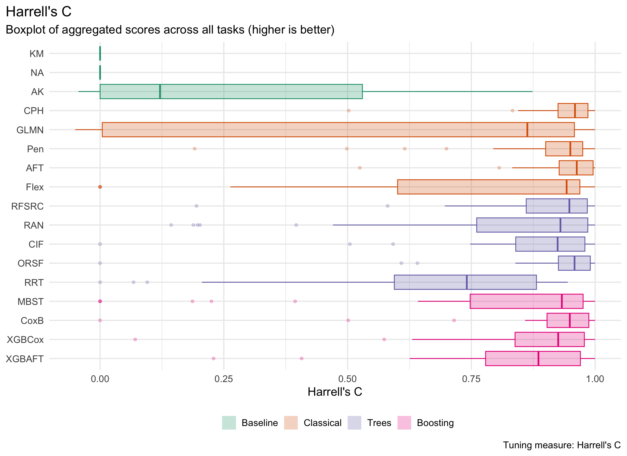
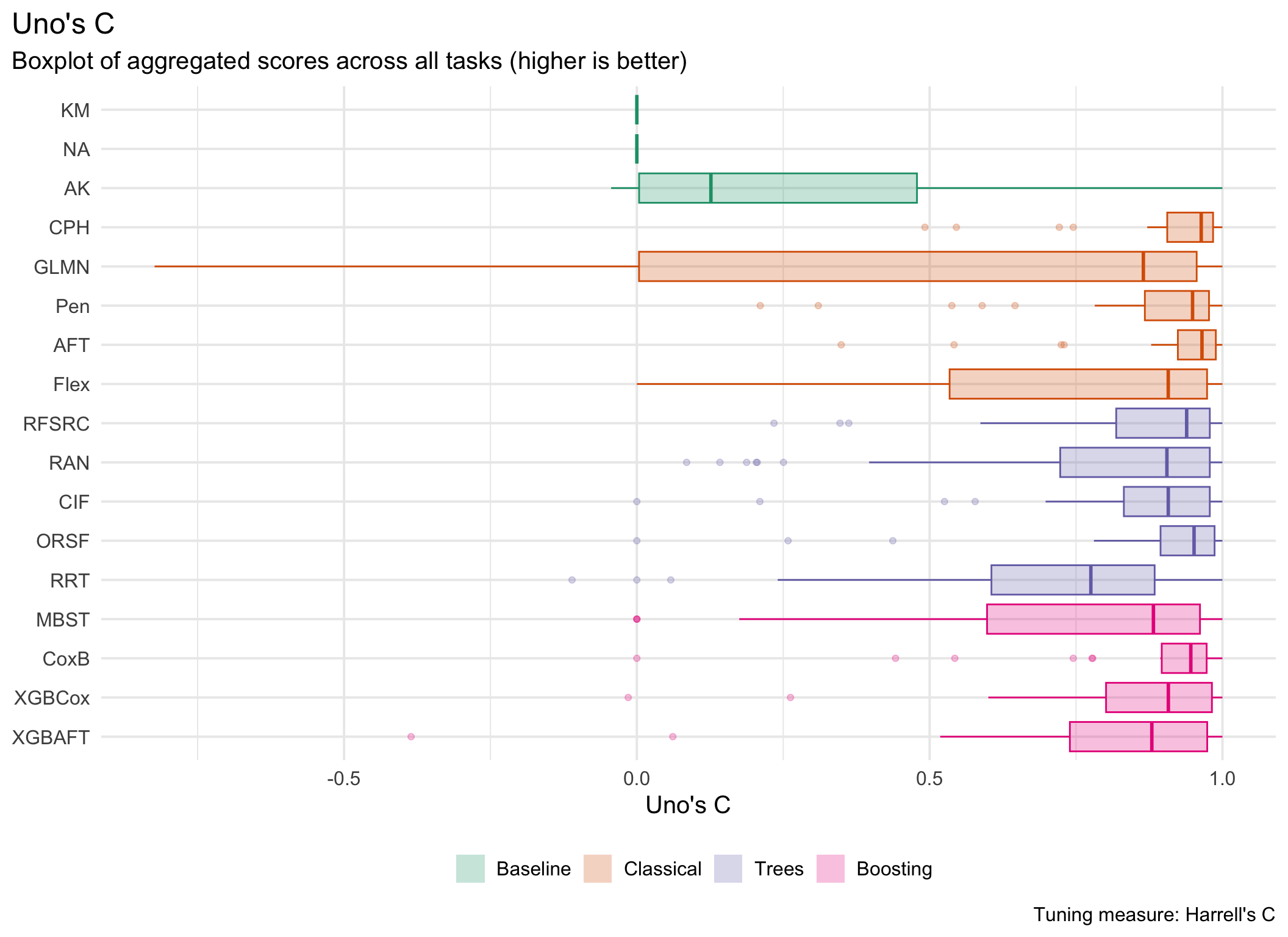
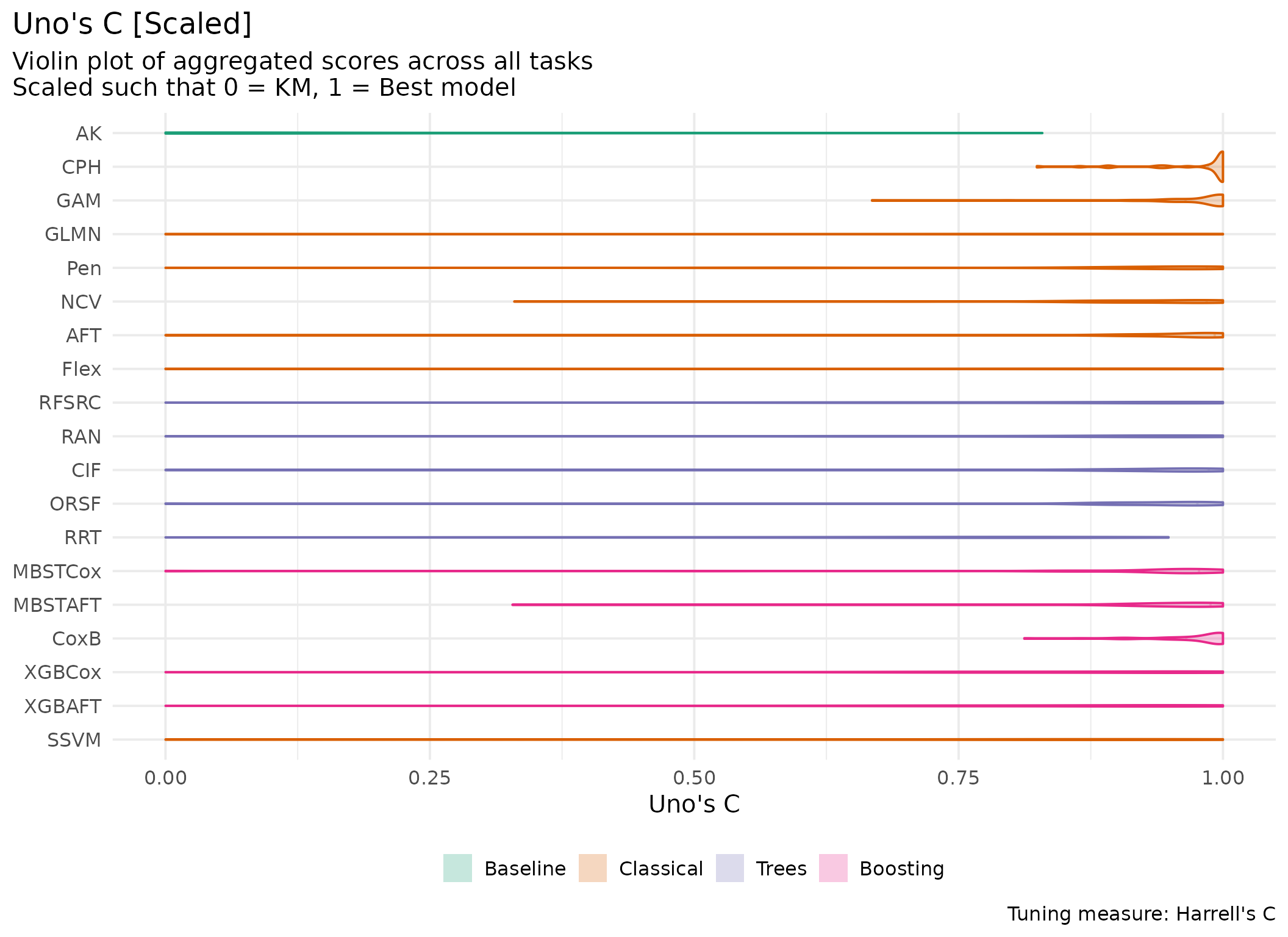
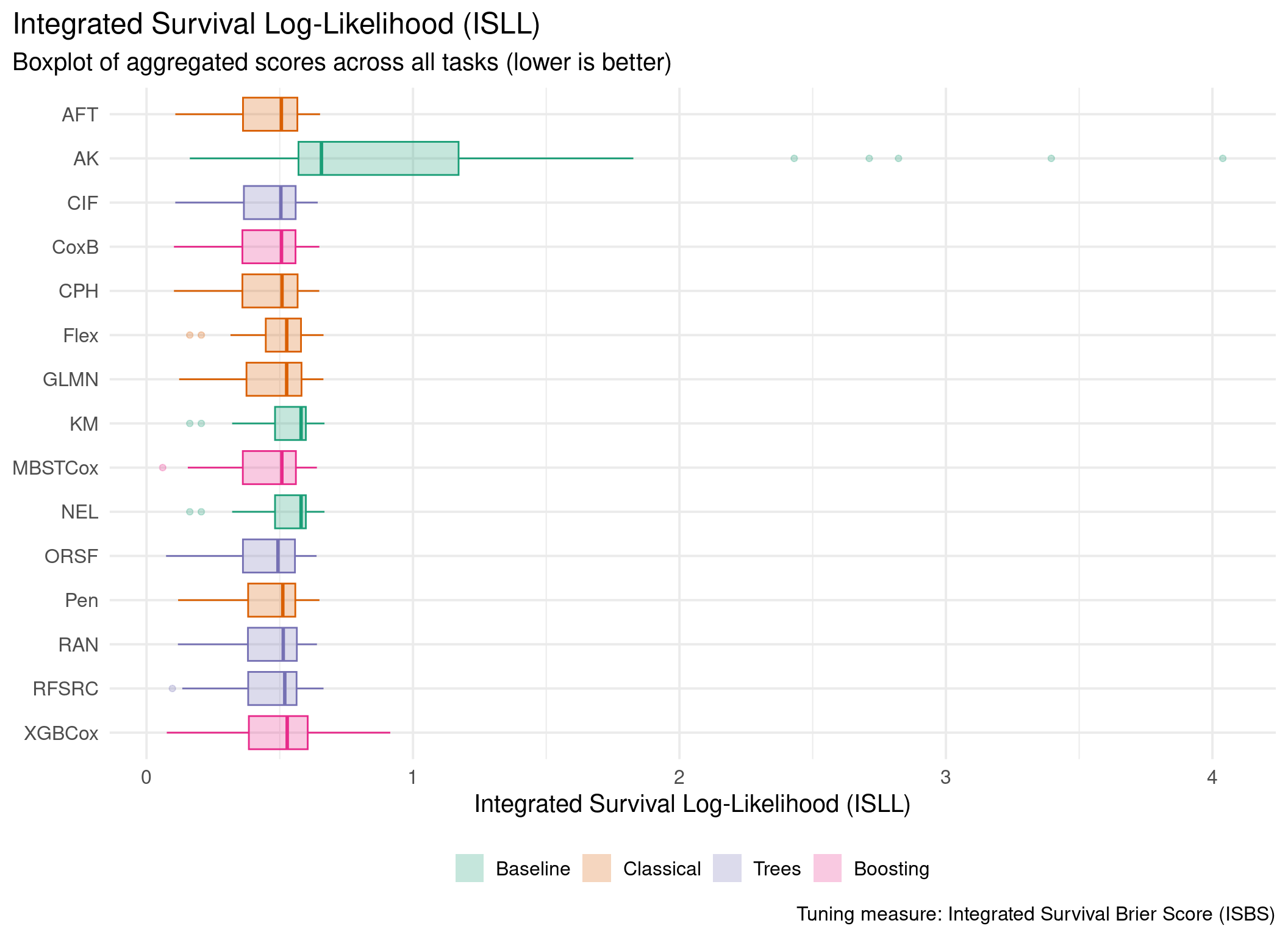
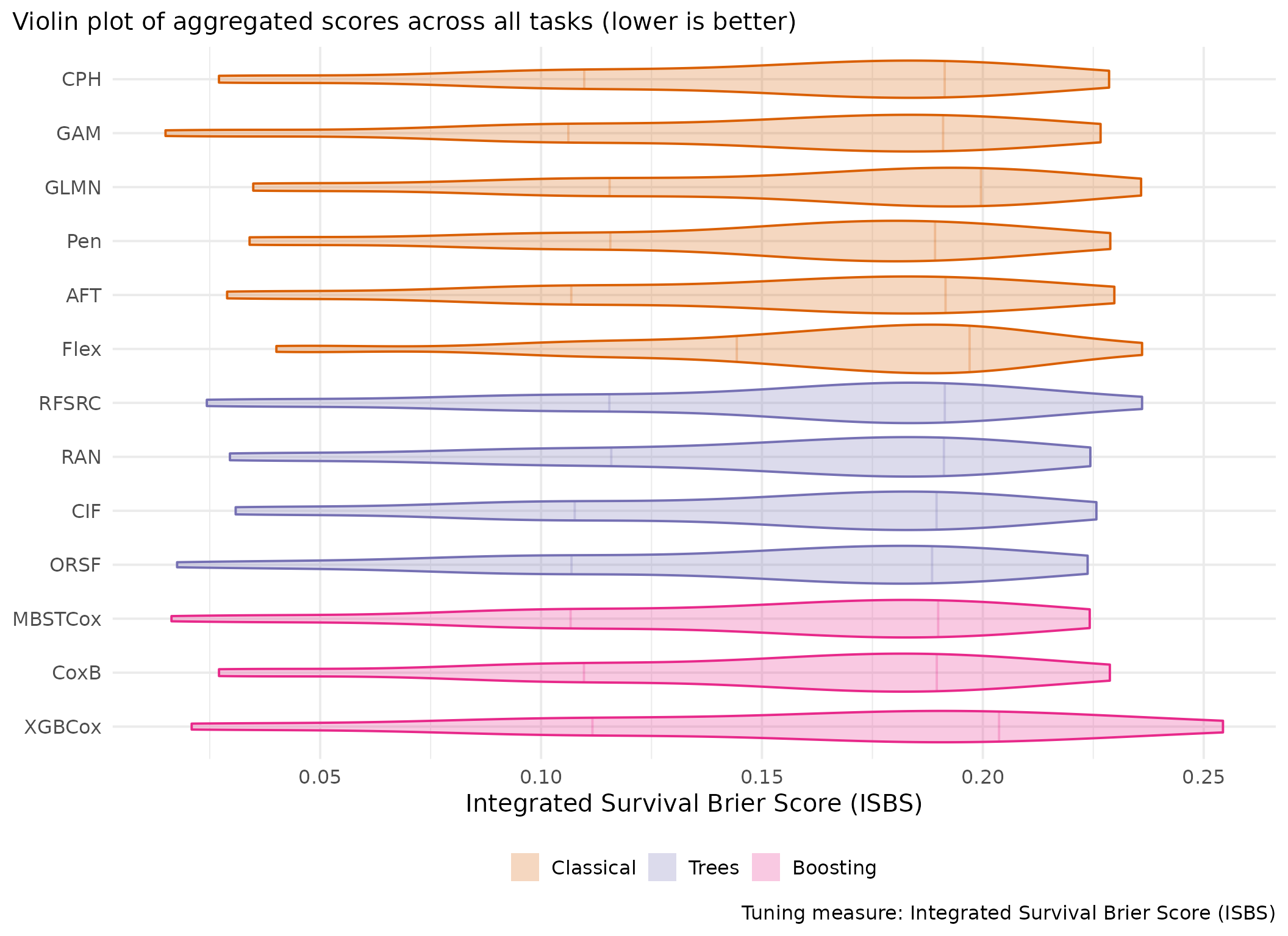
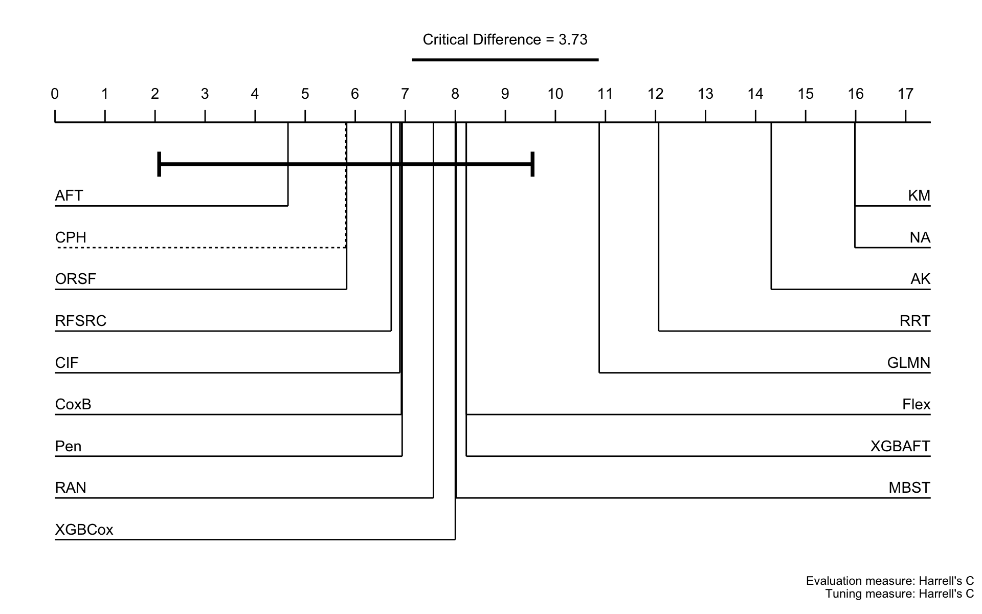
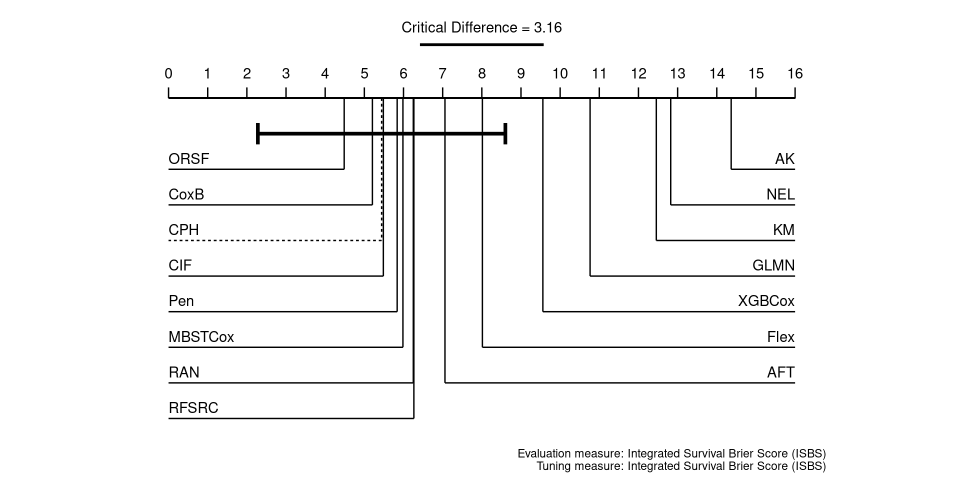
Burk et al. (2024)
  • Home
  • Results
  • Models, Data, Measures

On this page

  • Errros and elapsed time limits
  • Aggregated Results
    • Boxplots
  • Results per Dataset
    • Boxplots
    • Calibration
      • D-Calibration
      • Alpha-Calibration
    • Raw scores
  • Statistical Analysis
    • Global Friedman Test
    • Critical Difference Plots: Bonferroni-Dunn
  • Report an issue

This page gives an overview of the benchmark results, including scores aggregated across outer resampling iterations used for later statistical analysis and individual scores per dataset and model.

In general, results are divided by underlying tuning measure, i.e. harrel_c and isbs, with the former being a measure of discrimination and the latter a proper scoring rule.

Errros and elapsed time limits

The following table lists the number of errors in the outer resampling iterations per tuning measure (tuned). These errors were caused by the learner exceeding the time limit or exceeding memory limitations. We attempted to resubmit failing computational jobs with increased memory limits, yet in some cases the jobs still failed with more than 100GB of available memory, at which point we considered the learner/task combination to just be infeasible.

We note:

  • the affected learners were particularly slow or memory intensive for large tasks with many observations or a large number of unique time points, where the latter in particular appeared even more relevant than the number of observations.
  • the tasks below are most often those with many observations and unique time points (hdfail, child, check_times).

We therefore consider the errors to be a result of the learners’ complexity and the tasks’ size, given reasonable computational constraints.

Click to view table
Code
err_tbl <- scores |>
  dplyr::group_by(learner_id, task_id, tune_measure) |>
  dplyr::summarise(
    affected_iterations = sum(errors_cnt > 0),
    total_iterations = dplyr::n(),
    .groups = "drop"
  ) |>
  dplyr::filter(affected_iterations > 0) |>
  dplyr::mutate(
    error_rate = round(100 * affected_iterations / total_iterations, 1),
    errors_fmt = glue::glue("{affected_iterations} / {total_iterations} ({error_rate}%)")
  ) |>
  tidyr::pivot_wider(
    id_cols = c("learner_id", "task_id"),
    names_from = "tune_measure",
    values_from = "errors_fmt",
    values_fill = "—"
  )

err_tbl |>
  dplyr::select(-learner_id) |>
  kableExtra::kbl(
    col.names = c("Dataset", "Harrell's C", "ISBS"),
    caption = "Number of evaluations with errors of the total outer resampling iterations by tuning measure. (—) indicates there were no errors during evaluation, but possible during tuning."
  ) |>
  kableExtra::kable_styling() |>
  kableExtra::pack_rows(index = table(err_tbl$learner_id))
Number of evaluations with errors of the total outer resampling iterations by tuning measure. (—) indicates there were no errors during evaluation, but possible during tuning.
Dataset Harrell's C ISBS
AK
CarpenterFdaData 1 / 30 (3.3%) —
channing 1 / 30 (3.3%) 1 / 30 (3.3%)
child 3 / 3 (100%) 3 / 3 (100%)
e1684 — 3 / 30 (10%)
hdfail 3 / 3 (100%) 3 / 3 (100%)
lung — 8 / 30 (26.7%)
uis — 2 / 30 (6.7%)
veteran — 3 / 30 (10%)
CIF
child 3 / 3 (100%) 3 / 3 (100%)
hdfail 3 / 3 (100%) 3 / 3 (100%)
Flex
aids.id 10 / 30 (33.3%) —
check_times 3 / 3 (100%) 3 / 3 (100%)
child 3 / 3 (100%) 3 / 3 (100%)
dataFTR — 2 / 30 (6.7%)
hdfail 3 / 3 (100%) 3 / 3 (100%)
lung — 9 / 30 (30%)
nafld1 14 / 15 (93.3%) 14 / 15 (93.3%)
nwtco 15 / 15 (100%) 15 / 15 (100%)
support 3 / 3 (100%) 3 / 3 (100%)
wa_churn 15 / 15 (100%) 15 / 15 (100%)
GLMN
bladder0 — 1 / 30 (3.3%)
channing 1 / 30 (3.3%) —
check_times — 2 / 3 (66.7%)
cost — 12 / 30 (40%)
dataSTR — 2 / 30 (6.7%)
hdfail 3 / 3 (100%) —
std — 6 / 30 (20%)
uis — 4 / 30 (13.3%)
veteran 14 / 30 (46.7%) —
wbc1 4 / 30 (13.3%) —
MBSTAFT
hdfail — 2 / 3 (66.7%)
MBSTCox
child 3 / 3 (100%) 3 / 3 (100%)
dataSTR 1 / 30 (3.3%) —
hdfail 3 / 3 (100%) 3 / 3 (100%)
ORSF
child 3 / 3 (100%) 3 / 3 (100%)
cost — 1 / 30 (3.3%)
gbsg — 1 / 15 (6.7%)
hdfail 3 / 3 (100%) 3 / 3 (100%)
nafld1 9 / 15 (60%) 1 / 15 (6.7%)
uis 1 / 30 (3.3%) —
veteran — 1 / 30 (3.3%)
Pen
aids.id 9 / 30 (30%) 1 / 30 (3.3%)
bladder0 — 8 / 30 (26.7%)
channing — 1 / 30 (3.3%)
check_times 3 / 3 (100%) 3 / 3 (100%)
cost — 3 / 30 (10%)
dataSTR 3 / 30 (10%) 11 / 30 (36.7%)
hdfail 2 / 3 (66.7%) —
RAN
check_times 2 / 3 (66.7%) 3 / 3 (100%)
child 3 / 3 (100%) 3 / 3 (100%)
cost — 1 / 30 (3.3%)
hdfail 1 / 3 (33.3%) 1 / 3 (33.3%)
mgus 2 / 30 (6.7%) —
nafld1 9 / 15 (60%) 4 / 15 (26.7%)
RFSRC
check_times 3 / 3 (100%) 3 / 3 (100%)
child 3 / 3 (100%) 3 / 3 (100%)
colrec 2 / 3 (66.7%) 1 / 3 (33.3%)
nafld1 1 / 15 (6.7%) 2 / 15 (13.3%)
support 3 / 3 (100%) 2 / 3 (66.7%)
RRT
dataFTR — 5 / 30 (16.7%)
lung — 8 / 30 (26.7%)
metabric — 7 / 15 (46.7%)
nwtco — 7 / 15 (46.7%)
ova — 3 / 30 (10%)
tumor — 3 / 30 (10%)
SSVM
check_times — 3 / 3 (100%)
child — 3 / 3 (100%)
colrec — 3 / 3 (100%)
flchain — 11 / 15 (73.3%)
hdfail — 3 / 3 (100%)
nafld1 — 15 / 15 (100%)
nwtco — 8 / 15 (53.3%)
ova — 3 / 30 (10%)
support — 3 / 3 (100%)
wa_churn — 15 / 15 (100%)

Aggregated Results

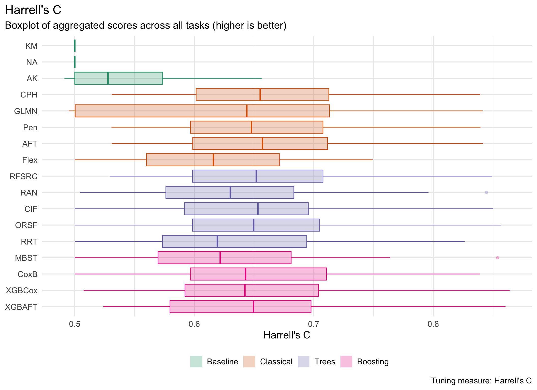
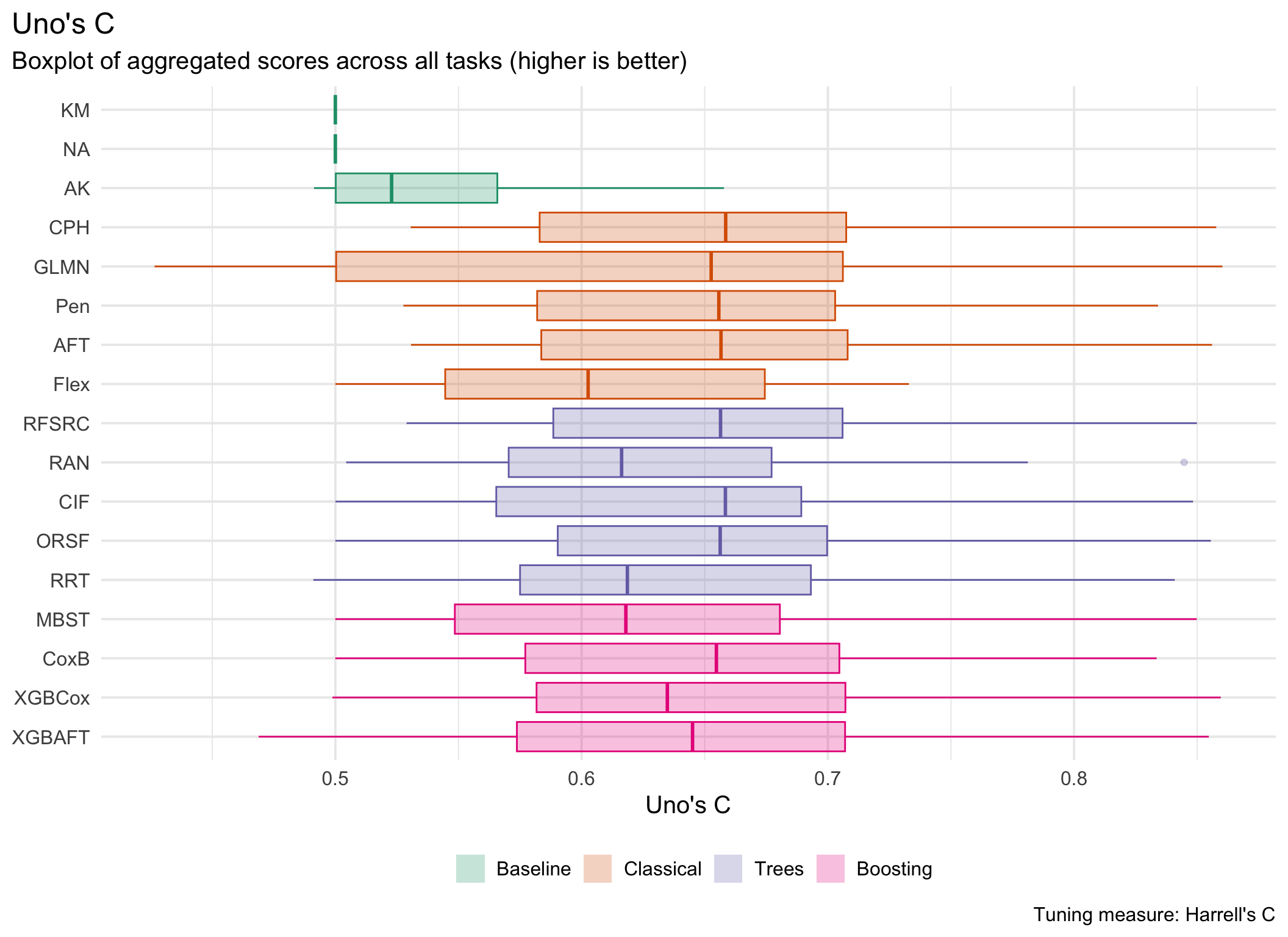
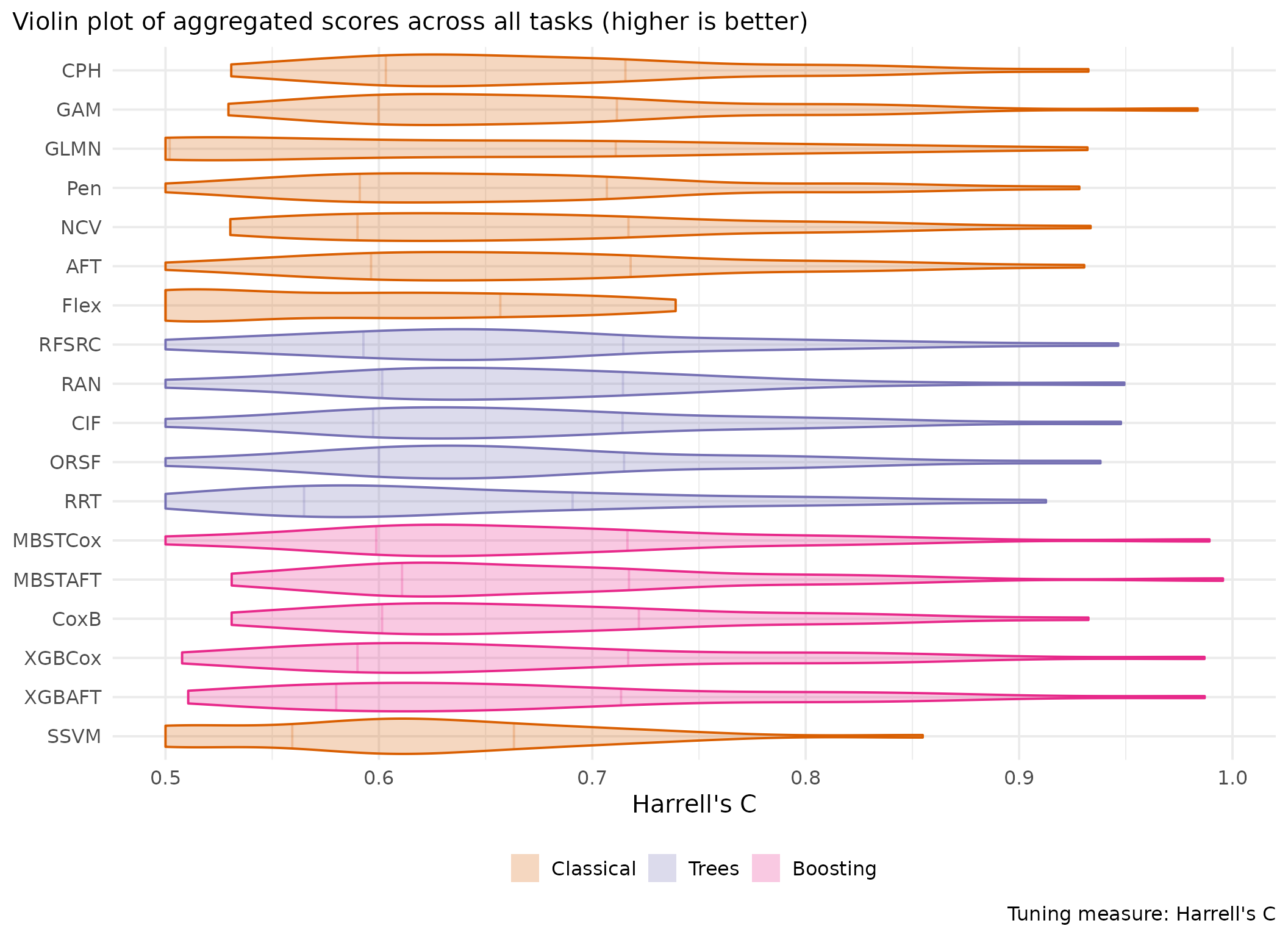
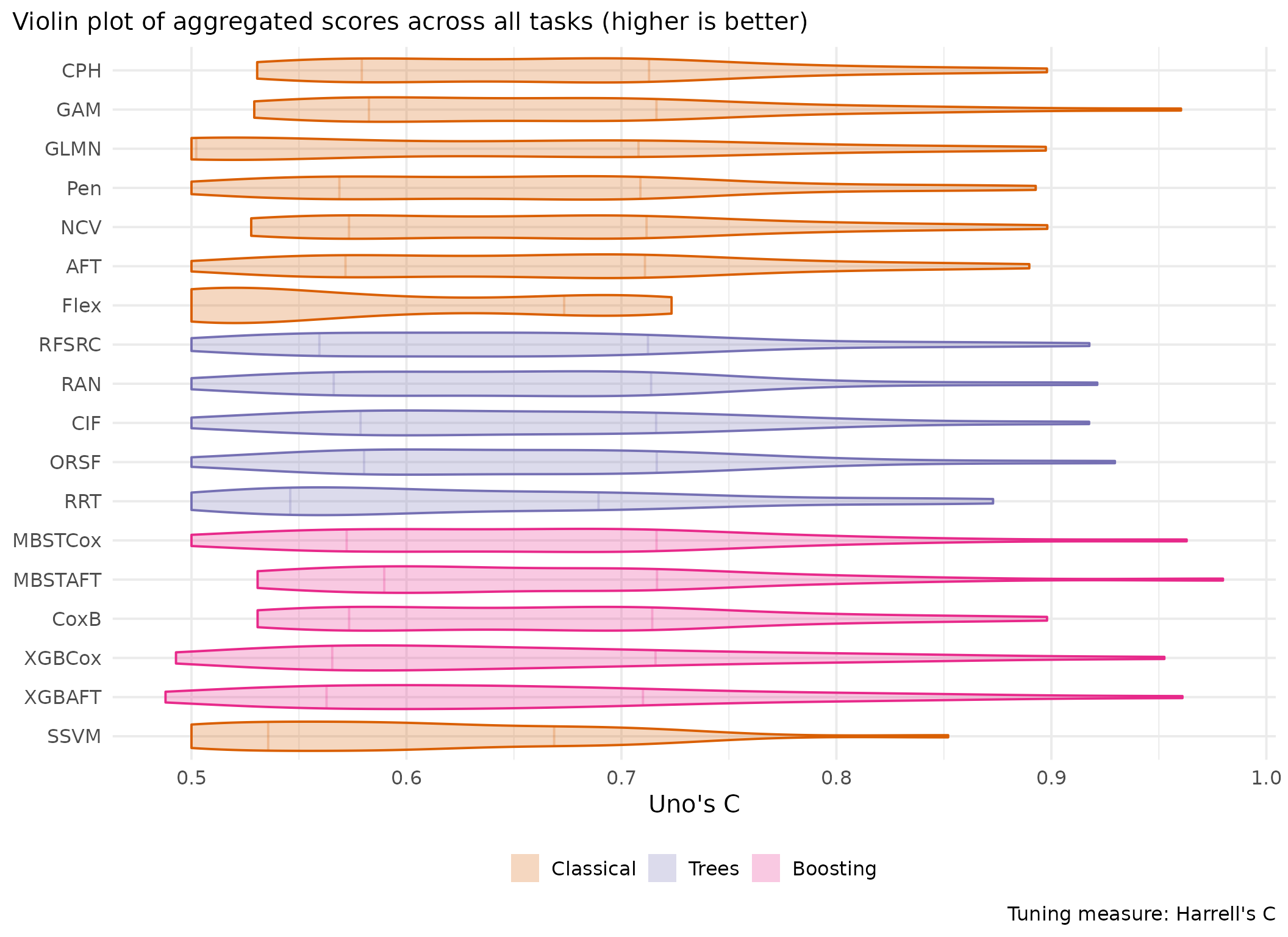
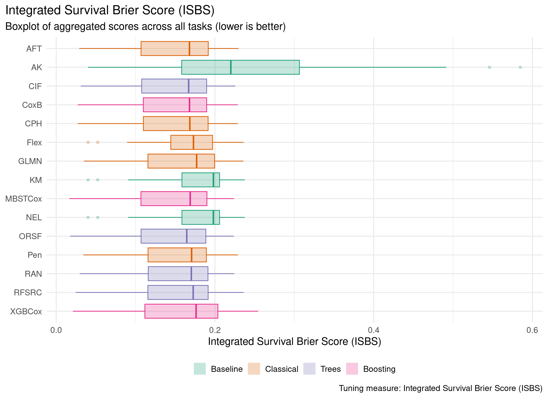
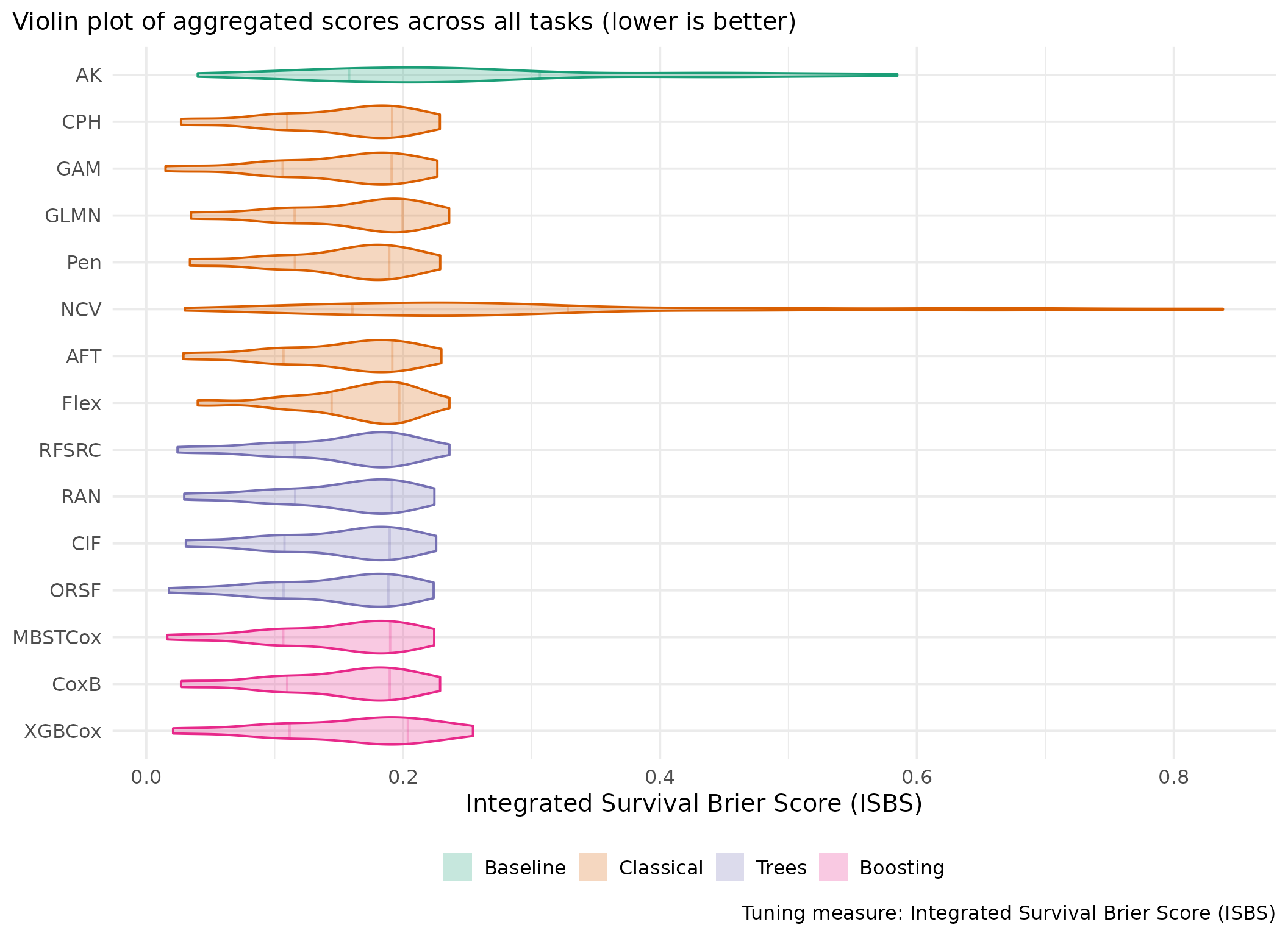
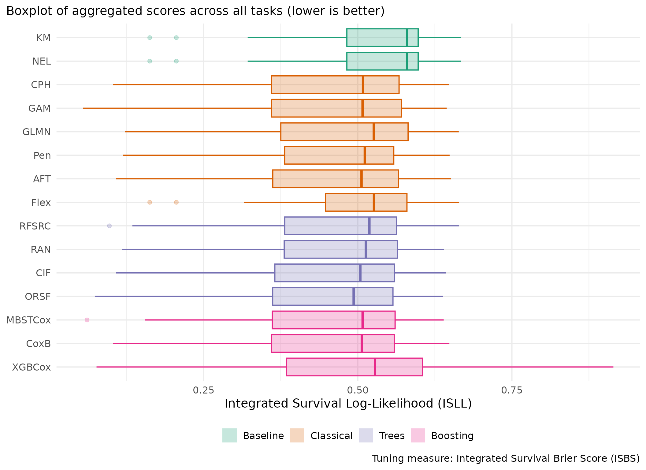
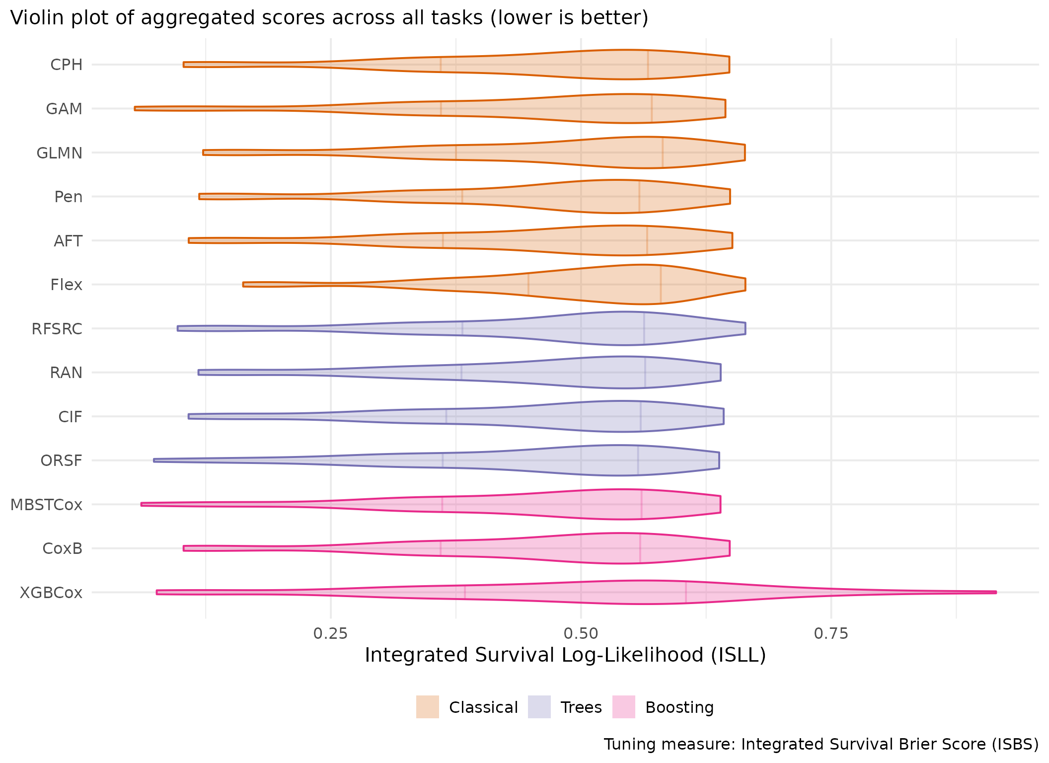
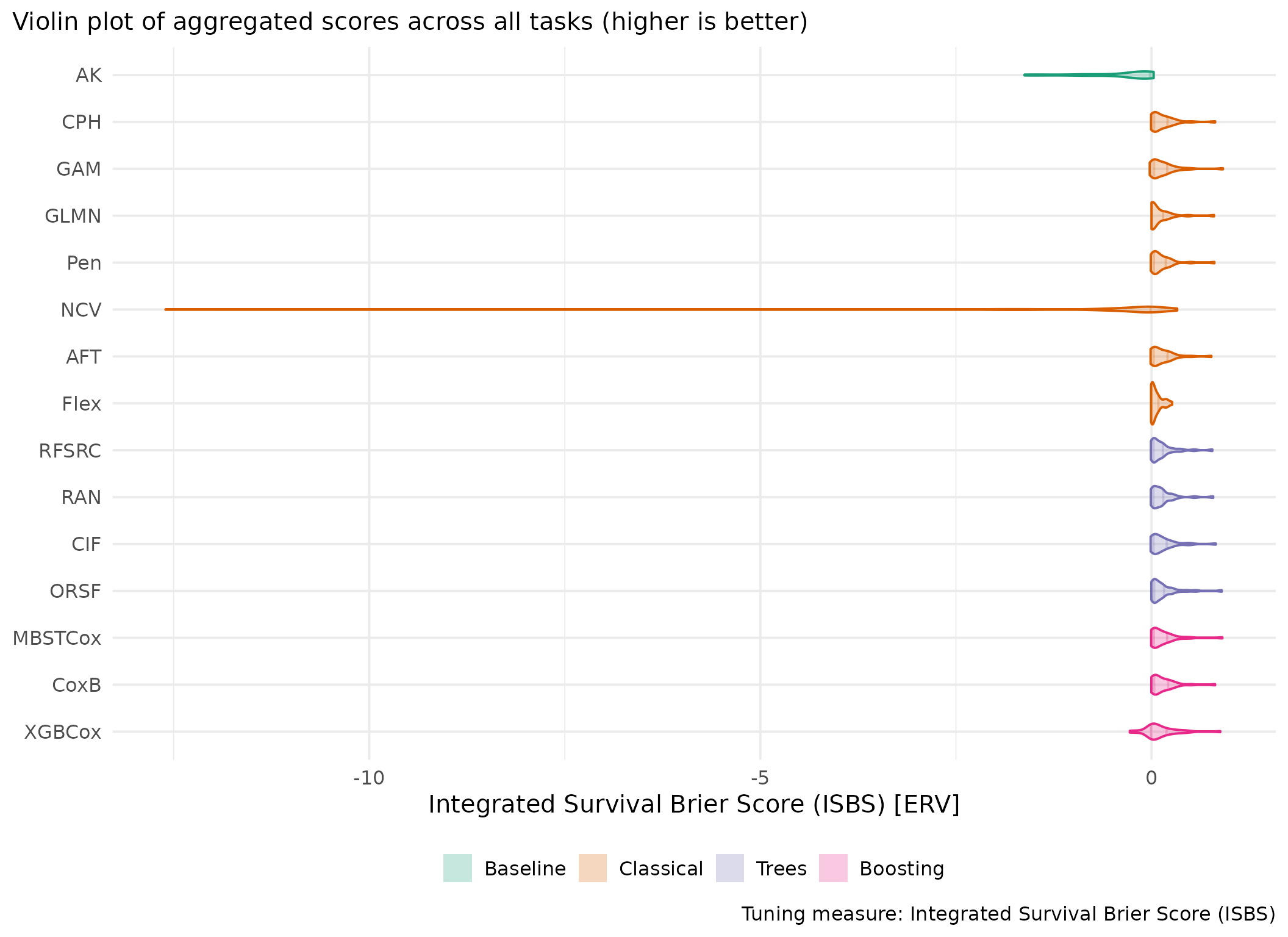
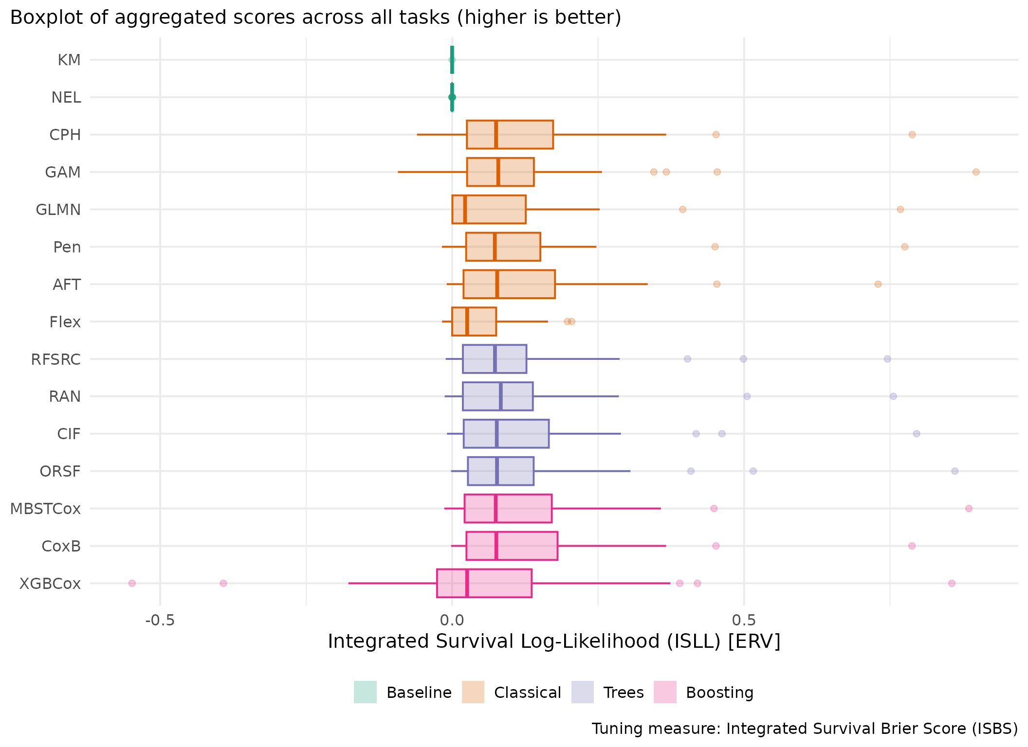
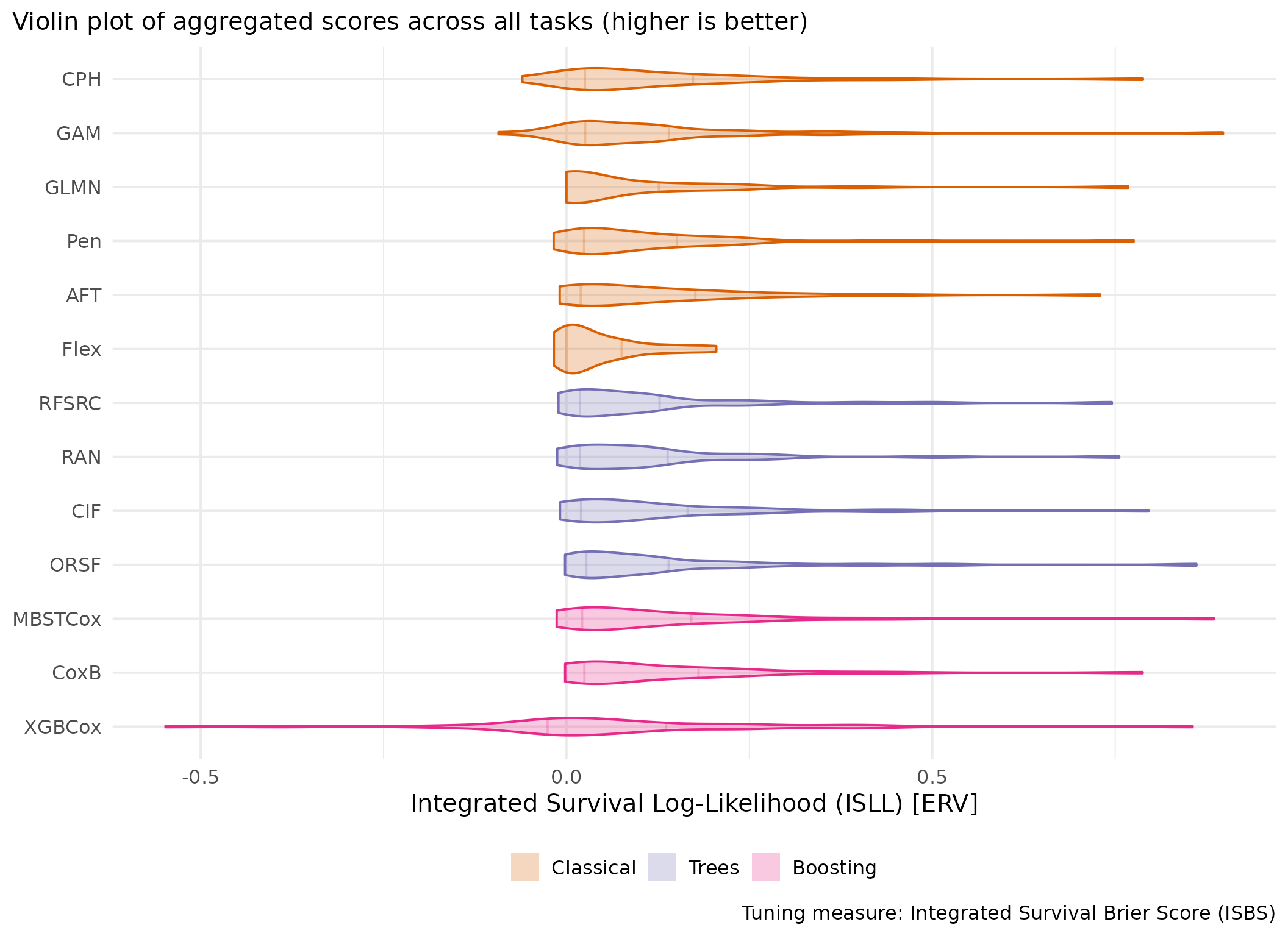
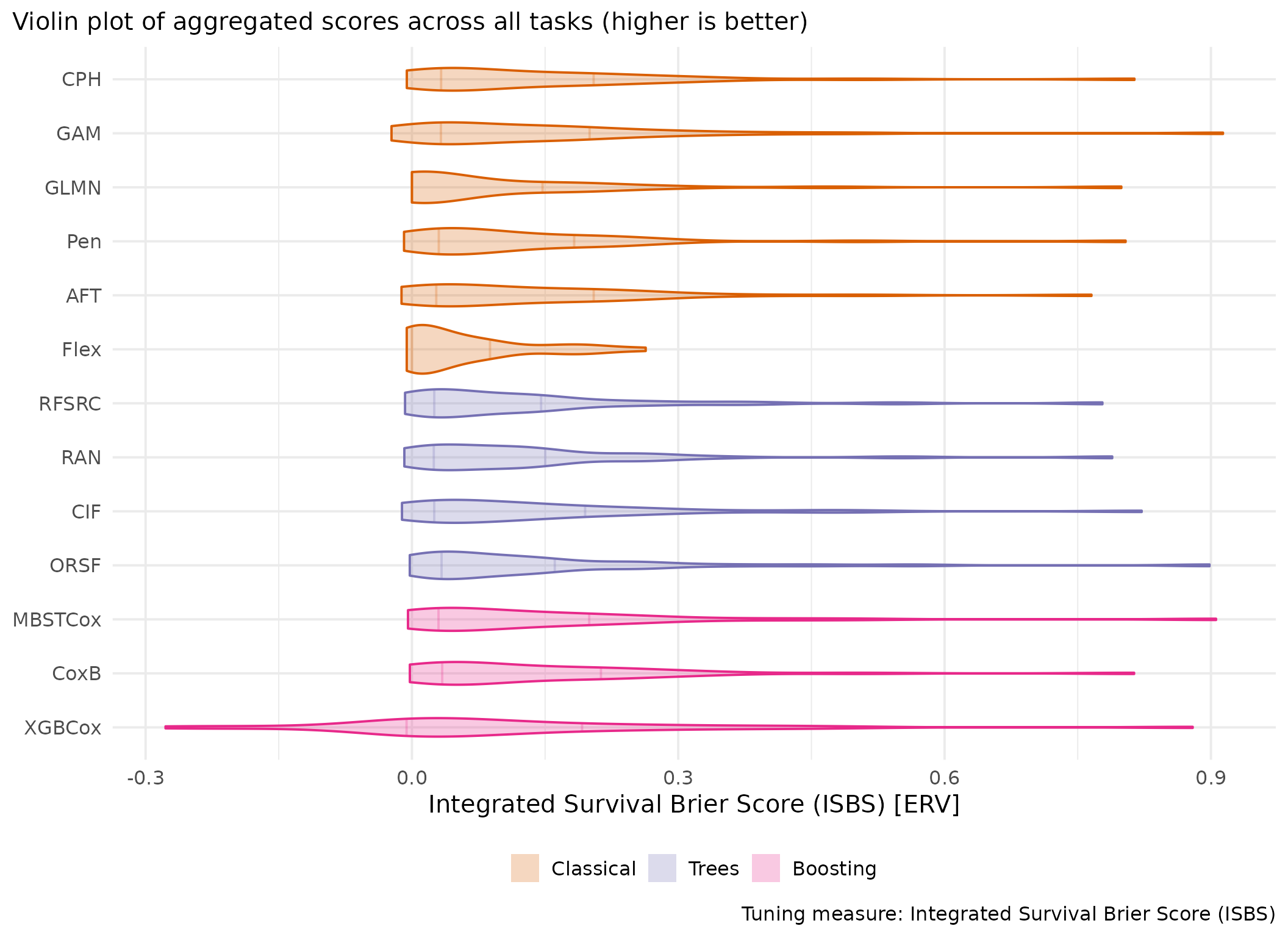
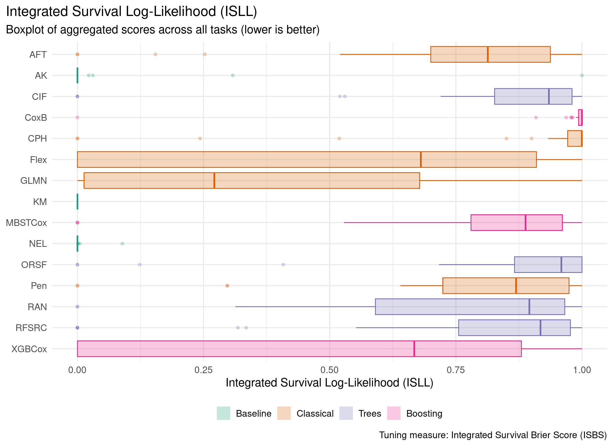
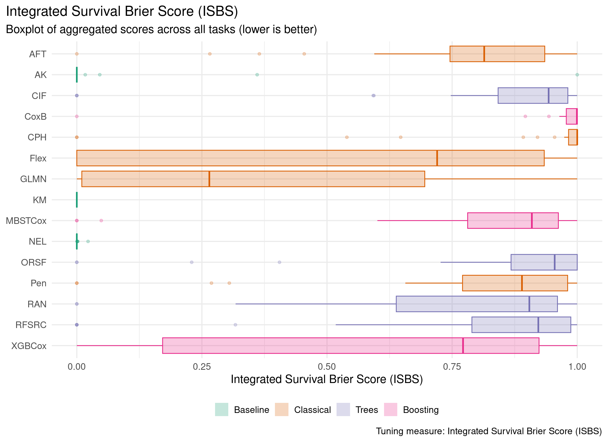
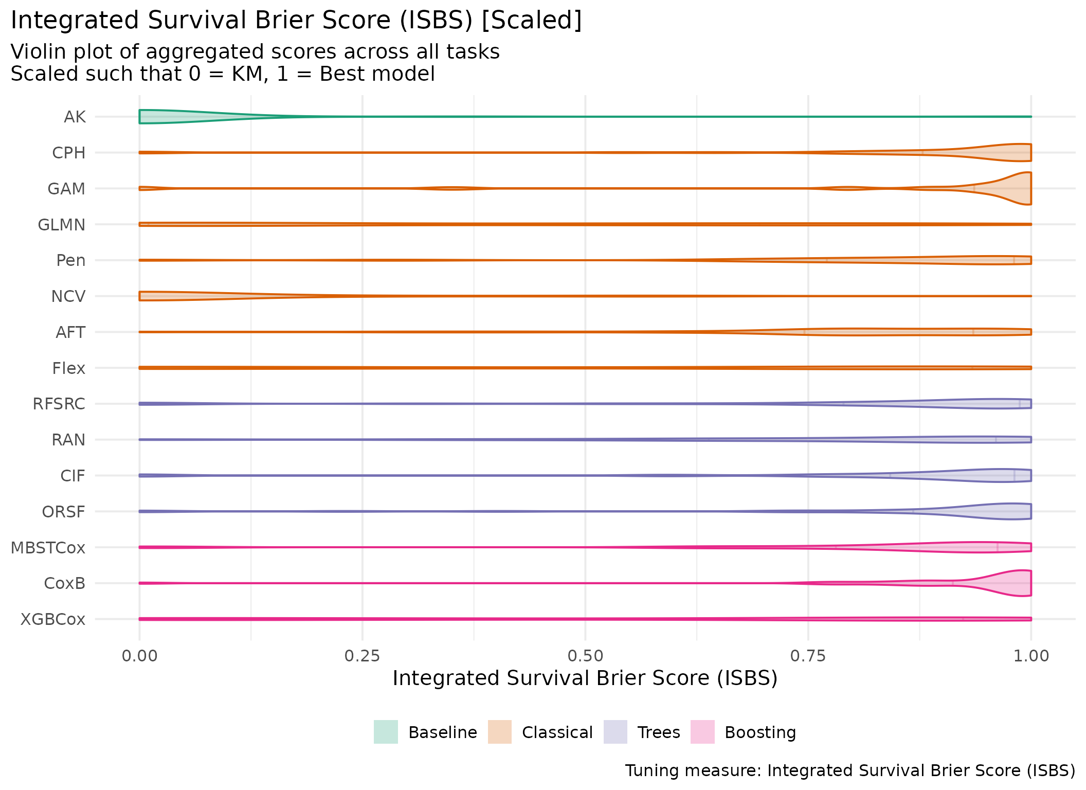
Averaged scores across outer resampling folds for each task and learner.

Boxplots

  • Harrell’s C
  • ISBS
Code
for (measure_id in msr_tbl[type == "Discrimination", id]) {
  plot_aggr_scores(
    aggr_scores,
    type = "box",
    eval_measure_id = measure_id,
    tuning_measure_id = "harrell_c",
    dodge = FALSE,
    flip = TRUE
  )
}

Harrell’s C (Scaled)

Code
for (measure_id in msr_tbl[type == "Discrimination", id]) {
  plot_aggr_scores(
    aggr_scores_scaled,
    type = "box",
    eval_measure_id = measure_id,
    tuning_measure_id = "harrell_c",
    dodge = FALSE,
    flip = TRUE
  ) %+%
    labs(
      title = glue::glue("{msr_tbl[id == measure_id, label]} [Scaled KM – Best]"),
      subtitle = "Boxplot of aggregated scores across all tasks scaled such that 0 = KM, 1 = Best model"
    )
}

Code
for (measure_id in msr_tbl[type == "Scoring Rule" & !erv, id]) {
  plot_aggr_scores(
    aggr_scores,
    type = "box",
    eval_measure_id = measure_id,
    tuning_measure_id = "isbs",
    dodge = FALSE,
    flip = TRUE
  )
}

ISBS (ERV)

Code
for (measure_id in msr_tbl[type == "Scoring Rule" & erv, id]) {
  plot_aggr_scores(
    aggr_scores,
    type = "box",
    eval_measure_id = measure_id,
    tuning_measure_id = "isbs",
    dodge = FALSE,
    flip = TRUE
  )
}

Scaled ISBS

Code
for (measure_id in msr_tbl[type == "Scoring Rule" & !erv, id]) {
  plot_aggr_scores(
    aggr_scores_scaled,
    type = "box",
    eval_measure_id = measure_id,
    tuning_measure_id = "isbs",
    dodge = FALSE,
    flip = TRUE
  ) %+%
    labs(
      title = glue::glue("{msr_tbl[id == measure_id, label]} [Scaled KM-Best]"),
      subtitle = "Boxplot of aggregated scores across all tasks scaled such that 0 = KM, 1 = Best model"
    )
}

Results per Dataset

Taking scores from the outer evaluation folds, see scores.[csv|rds].

Boxplots

  • Harrell’s C
  • ISBS
Code
for (measure_id in msr_tbl[type == "Discrimination", id]) {
  plot_scores(scores, eval_measure_id = measure_id, tuning_measure_id = "harrell_c", dodge = FALSE, flip = TRUE)
}
Code
for (measure_id in msr_tbl[type == "Scoring Rule" & !erv, id]) {
  plot_scores(scores, eval_measure_id = measure_id, tuning_measure_id = "isbs", dodge = FALSE, flip = TRUE)
}

Calibration

D-Calibration

Calculating p-values for D-Calibration as pchisq(score, 10 - 1, lower.tail = FALSE).

This represents more of a heuristic approach as an insignificant result implies a well-calibrated model, but a significant result does not necessarily imply a poorly calibrated model. Furthermore, there is no multiplicity correction applied due to the generally exploratory nature of the plots.

Code
aggr_scores |>
  dplyr::filter(grepl("isbs", tune_measure)) |>
  dplyr::mutate(
    dcalib_p = pchisq(dcalib, 10 - 1, lower.tail = FALSE),
    dcalib_label = fifelse(dcalib_p < 0.05, "X", "")
  ) |>
  ggplot(aes(
    x = forcats::fct_reorder(learner_id, dcalib_p),
    y = forcats::fct_rev(task_id),
    fill = dcalib_p
  )) +
  geom_tile(color = "#EEEEEE") +
  geom_text(aes(label = dcalib_label), color = "white", size = 3) +
  # scale_fill_manual(values = c(`TRUE` = "red", `FALSE` = "blue"), labels = c(`TRUE` = "Signif.", `FALSE` = "Not Signif.")) +
  scale_fill_viridis_c(breaks = seq(0, 1, .1)) +
  guides(
    x = guide_axis(n.dodge = 2),
    fill = guide_colorbar(
      title.vjust = .8,
      barwidth = unit(200, "pt")
    )
  ) +
  labs(
    title = "D-Calibration p-values by task and learner",
    subtitle = glue::glue(
      "Models tuned on {msr_tbl[id == 'isbs', label]}\n",
      "Learners ordered by average p-value. X denotes p < 0.05"
    ),
    y = "Task",
    x = "Learner",
    color = NULL,
    fill = "p-value"
  ) +
  theme_minimal() +
  theme(
    legend.position = "bottom",
    plot.title.position = "plot",
    panel.grid.major.y = element_blank(),
    panel.grid.minor.y = element_blank(),
    panel.spacing.x = unit(5, "mm"),
    panel.background = element_rect(fill = "#EEEEEE", color = "#EEEEEE")
  )

Alpha-Calibration

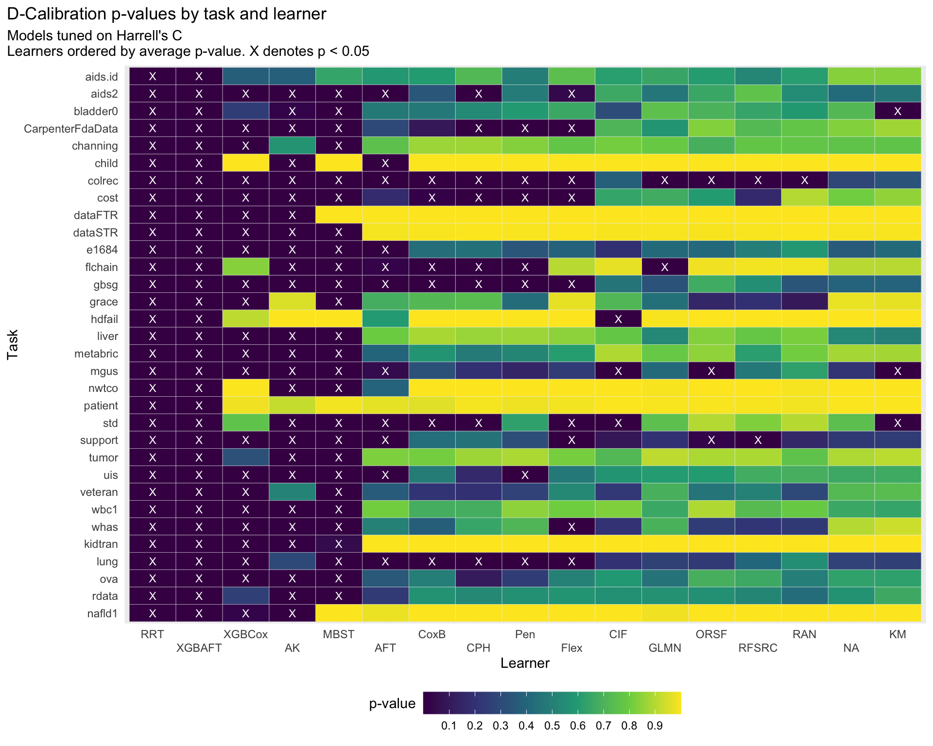
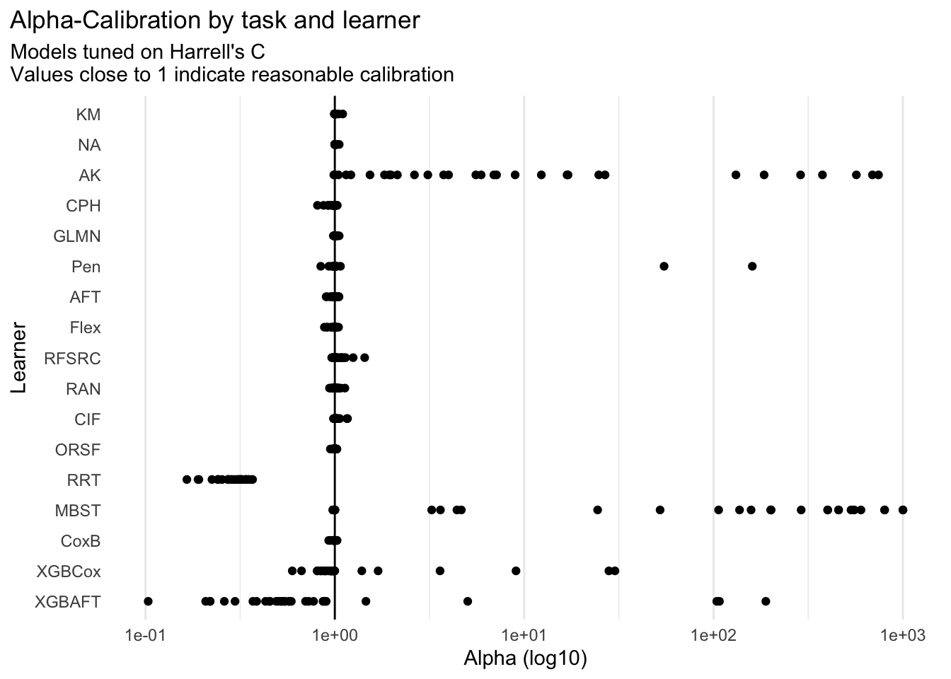
For this measure, calibration is indicated by a score close to 1.

Code
ggplot(aggr_scores[grepl("isbs", tune_measure)], aes(y = forcats::fct_rev(learner_id), x = alpha_calib)) +
  geom_point() +
  geom_vline(xintercept = 1) +
  scale_x_log10() +
  labs(
    title = "Alpha-Calibration by task and learner",
    subtitle = glue::glue(
      "Models tuned on {msr_tbl[id == 'isbs', label]}\n",
      "Values close to 1 indicate reasonable calibration"
    ),
    y = "Learner",
    x = "Alpha (log10)"
  ) +
  theme_minimal() +
  theme(
    legend.position = "bottom",
    plot.title.position = "plot",
    panel.grid.major.y = element_blank(),
    panel.grid.minor.y = element_blank()
    # panel.spacing.x = unit(5, "mm"),
    # panel.background = element_rect(fill = "#EEEEEE", color = "#EEEEEE")
  )

Raw scores

Variable Type Description
task_id fct Dataset name, e.g. veteran
learner_id fct Model / learner name, e.g. RAN for ranger
harrell_c dbl Evaluation measure score
uno_c dbl Evaluation measure score
isll dbl Evaluation measure score
isll_erv dbl Evaluation measure score
isbs dbl Evaluation measure score
isbs_erv dbl Evaluation measure score
dcalib dbl Evaluation measure score
alpha_calib dbl Evaluation measure score
tune_measure chr Tuning measure, one of harrell_c, isbs
learner_group fct Model / learner group, one of “Baseline”, “Classical”m “Trees”, “Boosting”
Code
#|
aggr_scores |>
  dplyr::mutate(dplyr::across(dplyr::where(is.numeric), \(x) round(x, 3))) |>
  dplyr::arrange(task_id, learner_id) |>
  reactable::reactable(
    sortable = TRUE,
    filterable = TRUE,
    searchable = TRUE,
    defaultPageSize = 30
  )

Statistical Analysis

Global Friedman Test

  • Harrell’s C
  • ISBS
Code
bma_harrell_c$friedman_test(p.adjust.method = "holm") |>
  tablify()
X2 df p.value p.adj.value p.signif
harrell_c 307.4551 18 1.407696e-54 0 ***
uno_c 297.5853 18 1.510542e-52 0 ***
Code
bma_isbs$friedman_test(p.adjust.method = "holm") |>
  tablify()
X2 df p.value p.adj.value p.signif
isll 243.7411 14 5.650619e-44 0 ***
isll_erv 244.186 14 4.572789e-44 0 ***
isbs 244.2825 14 4.367824e-44 0 ***
isbs_erv 243.612 14 6.008274e-44 0 ***
dcalib 126.2515 14 3.726951e-20 0 ***
alpha_calib 218.4822 14 9.004844e-39 0 ***

Critical Difference Plots: Bonferroni-Dunn

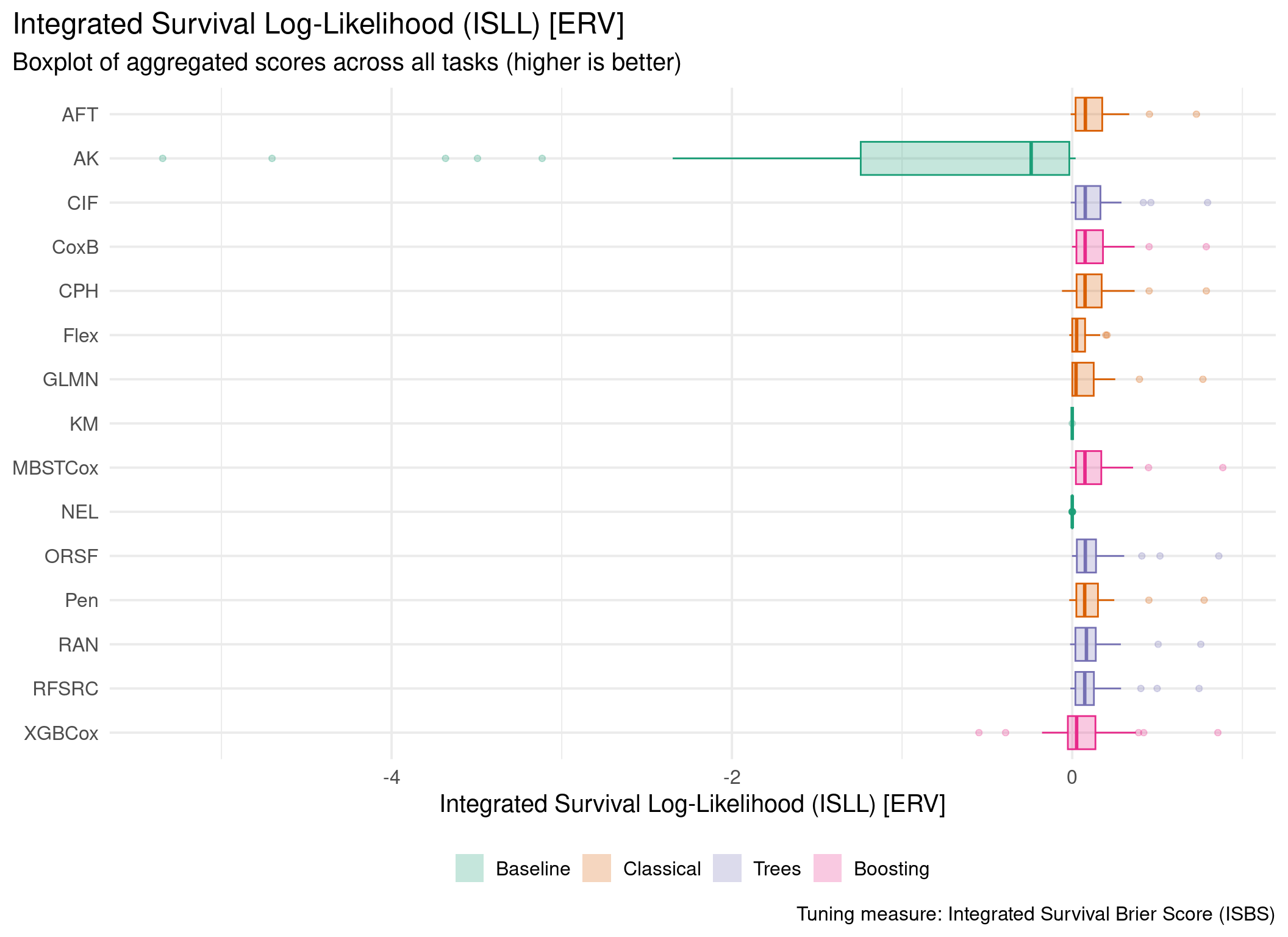
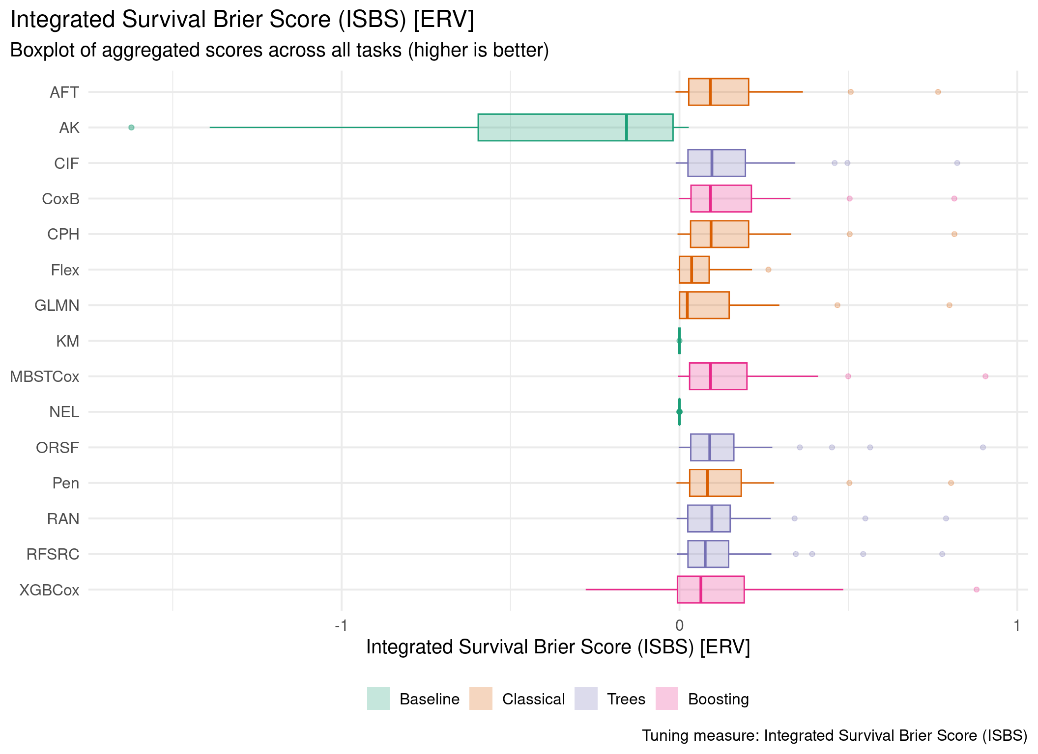
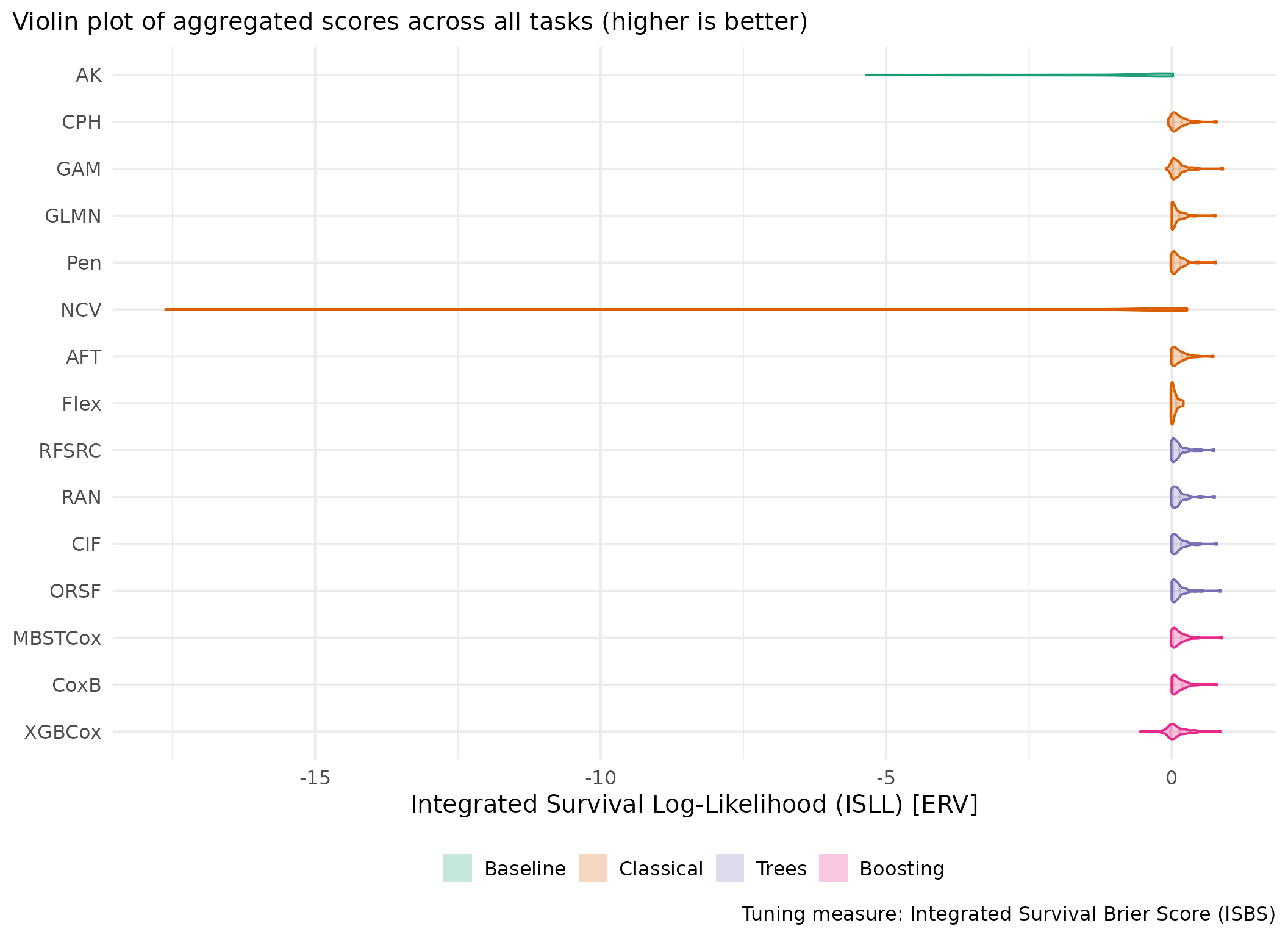
Using Cox (CPH) as baseline for comparison, these represent the primary result of the benchmark.

  • Harrell’s C
  • ISBS
Code
cd_ratio = 10 / 11

plot_bma(
  bma = bma_harrell_c,
  type = "cd_bd",
  measure_id = "harrell_c",
  tuning_measure_id = "harrell_c",
  ratio = cd_ratio,
  baseline = "CPH"
)
Warning in geom_segment(aes(x = 0, xend = max(rank) + 1, y = 0, yend = 0)): All aesthetics have length 1, but the data has 19 rows.
ℹ Please consider using `annotate()` or provide this layer with data containing
  a single row.

Code
plot_bma(
  bma = bma_isbs,
  type = "cd_bd",
  measure_id = "isbs",
  tuning_measure_id = "isbs",
  ratio = cd_ratio,
  baseline = "CPH"
)
Warning in geom_segment(aes(x = 0, xend = max(rank) + 1, y = 0, yend = 0)): All aesthetics have length 1, but the data has 15 rows.
ℹ Please consider using `annotate()` or provide this layer with data containing
  a single row.

  • Report an issue